Multiple joins are one of the toughest SQL concepts – in this post we’ll decode them and review some common pitfalls.
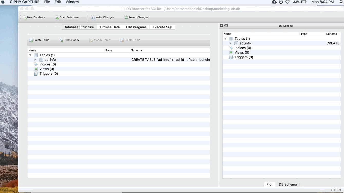
One of the best ways to learn is with an example. If you’d like to follow along, you can download this zip file that contains the three tables as .csv files here, and import them into DB Browser for SQLite. Read my post on how to use SQLite Browser here.
Say you work on the marketing team at a software company. Your database has the following tables.
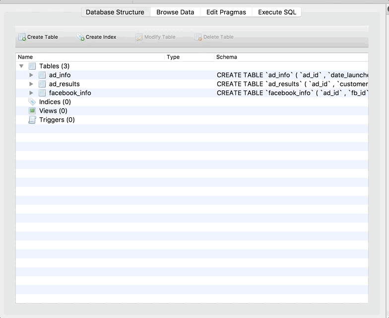
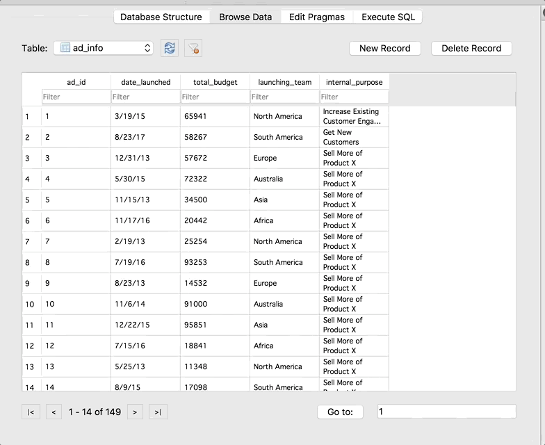
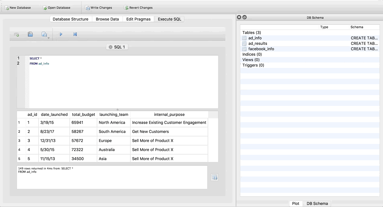
ad_info
Each row represents a unique campaign your company has run. All campaigns are included in this table.
fb_info
Each row represents a unique Facebook campaign. Only Facebook campaigns will show up in this table!
ad_results
Each row represents a unique campaign your company has run. All campaigns are included in this table.
Your boss asks you: what percentage of ad campaigns that were launched by the Europe or Australia teams and had success scores above 4 were Facebook campaigns?
To answer this question, we need to do a few things. Let’s break it down:
Filter results so we are only seeing European and Australian campaigns that had success scores above 4. We’ll do this in the WHERE clause. Don’t pay too much attention to this part for this example – we’re doing this to establish why we need all three tables, but the point of this example is to understand the joins. I’m not trying to trick anyone with the WHERE clause 🙂
Join the tables together so all the information is in one place.
Get the percentage of these specific campaigns that were Facebook campaigns. To do that, we’re going to count the number of rows in our result that have any information in the fb_information columns, and divide by the total number of rows in the result.
Okay, now we have all of the information we need to get started. You go back to your desk and you think “hmmmm…. I’m not sure how to do this.” We’re going to go through a few incorrect answers first before we look at the correct one so you can understand why the correct one is the right way to approach the problem.
Attempt 1: All Inner Joins
So, first you try all inner joins. Here’s a graphical representation of the joins:
A box represents the table
—- a line represents an inner join
and an arrow represents a left outer join.
And this is what the query looks like. I chose only to select the columns we need to answer the question, plus a few extras in the SELECT statement because if I selected all the columns, the table would be too large to fit easily into this webpage. But, for your own practice, you could do SELECT * if you want to see all the columns.
SELECT ad_info.ad_id, launching_team, fb_id, impressions, unique_reach, unique_clicks, engagement_rate, success_score
FROM ad_info INNER JOIN facebook_info
ON facebook_info.ad_id = ad_info.ad_id
INNER JOIN ad_results ON ad_results.ad_id = ad_info.ad_id
WHERE success_score > 4 AND launching_team IN ('Europe', 'Australia');
And finally, this is the result it produces:
Result:
| ad_id | launching_team | fb_id | impressions | unique_reach | unique_clicks | engagement_rate | success_score |
|---|
| 9 | Europe | fb-7647 | 5346 | 3713 | 3054 | 0.822515486 | 7 |
| 15 | Europe | fb-8982 | 9603 | 9508 | 5075 | 0.533761043 | 6 |
| 16 | Australia | fb-3763 | 9997 | 6854 | 5107 | 0.745112343 | 5 |
| 22 | Australia | fb-2011 | 3636 | 2464 | 1614 | 0.655032468 | 6 |
| 27 | Europe | fb-7448 | 2677 | 1702 | 1394 | 0.819036428 | 7 |
| 33 | Europe | fb-1526 | 7135 | 4185 | 4143 | 0.989964158 | 5 |
| 39 | Europe | fb-6513 | 1018 | 862 | 699 | 0.810904872 | 7 |
| 40 | Australia | fb-3680 | 8755 | 5785 | 5212 | 0.900950735 | 8 |
| 52 | Australia | fb-1584 | 4808 | 4409 | 2750 | 0.6237242 | 5 |
| 124 | Australia | fb-3866 | 8283 | 8209 | 4372 | 0.532586186 | 6 |
| 130 | Australia | fb-2977 | 2964 | 2878 | 2556 | 0.888116748 | 10 |
| 135 | Europe | fb-8359 | 6316 | 5308 | 3758 | 0.707987943 | 8 |
| 136 | Australia | fb-9569 | 2174 | 2078 | 1813 | 0.872473532 | 7 |
| 142 | Australia | fb-1790 | 7966 | 5743 | 5186 | 0.903012363 | 8 |
| 147 | Europe | fb-2933 | 4202 | 3030 | 2887 | 0.952805281 | 5 |
Remember, we are looking for the number of rows with data in the Facebook columns (fb_id, impressions, unique_reach, unique_clicks, engagement_rate) divided by the total number of rows in the result. This result looks like 100% of the European and Australian campaigns with a success_score greater than 4 were Facebook campaigns because all of the rows in the result have values in the Facebook columsn.
That should set off a red flag! Whenever you get something like this (100%, 0 rows, etc.) you should double-check your work. Remember, the scariest thing in SQL is not an error, but an incorrect result that we think is correct! What actually happened here is we’ve eliminated all of the non-Facebook European and Australian campaigns with success scores greater than 4.
Before I explain why, there are a few very important things to understand.
Table order doesn’t matter for ALL inner joins or ALL outer joins.
When you are doing all inner joins or all outer joins, whether you are joining 3 tables or 300, the order of the joins does not matter. Think back to the definition of the joins (check out this blog post for a refresher). Inner joins only keep what the tables have in common. So it doesn’t matter if I switch the order of the tables, I’ll still get a result that only contins rows that all tables have in common. An outer join will keep all rows from all tables, no matter what. So again, it doesn’t matter if I switch the order of the tables because SQL will always keep all rows.
How does SQL process this join?
It’s not the way it looks. First, it takes the entire ad_info table and inner joins it to the facebook_info table, and gets that result. Then it takes THAT RESULT and inner joins it to the ad_results table! So it’s not ad_info joined to facebook_info, and then facebook_info joined to ad_results. It’s the RESULT of ad_info-Inner-Join-facebook_info joined to ad_results.
It’s like you’re creating a cumulative table (but not always one that’s getting larger, it dependso n the type of JOINs you are doing). This makes multiple joins more difficult, because SQL will not show you the result of each join. You have to have an idea of what each result looks like at each
Therefore, the reason we got 100% is because the only thing these tables have in common is Facebook campaigns, since that is all that is in the facebook_info table. So, all inner joins is not the way to go.
Attempt 2: Mixed Joins Starting with facebook_info
Now let’s say we start with the facebook_info table, do a left outer join on the ad_info table next, and then an inner join to the ad_results table.
SELECT ad_info.ad_id, launching_team, fb_id, impressions, unique_reach, unique_clicks, engagement_rate, success_score
FROM facebook_info LEFT JOIN ad_info
ON facebook_info.ad_id = ad_info.ad_id
INNER JOIN ad_results ON ad_results.ad_id = ad_info.ad_id
WHERE success_score > 4 AND launching_team IN ('Europe', 'Australia');
Result:
| ad_id | launching_team | fb_id | impressions | unique_reach | unique_clicks | engagement_rate | success_score |
|---|
| 9 | Europe | fb-7647 | 5346 | 3713 | 3054 | 0.822515486 | 7 |
| 15 | Europe | fb-8982 | 9603 | 9508 | 5075 | 0.533761043 | 6 |
| 16 | Australia | fb-3763 | 9997 | 6854 | 5107 | 0.745112343 | 5 |
| 22 | Australia | fb-2011 | 3636 | 2464 | 1614 | 0.655032468 | 6 |
| 27 | Europe | fb-7448 | 2677 | 1702 | 1394 | 0.819036428 | 7 |
| 33 | Europe | fb-1526 | 7135 | 4185 | 4143 | 0.989964158 | 5 |
| 39 | Europe | fb-6513 | 1018 | 862 | 699 | 0.810904872 | 7 |
| 40 | Australia | fb-3680 | 8755 | 5785 | 5212 | 0.900950735 | 8 |
| 52 | Australia | fb-1584 | 4808 | 4409 | 2750 | 0.6237242 | 5 |
| 124 | Australia | fb-3866 | 8283 | 8209 | 4372 | 0.532586186 | 6 |
| 130 | Australia | fb-2977 | 2964 | 2878 | 2556 | 0.888116748 | 10 |
| 135 | Europe | fb-8359 | 6316 | 5308 | 3758 | 0.707987943 | 8 |
| 136 | Australia | fb-9569 | 2174 | 2078 | 1813 | 0.872473532 | 7 |
| 142 | Australia | fb-1790 | 7966 | 5743 | 5186 | 0.903012363 | 8 |
| 147 | Europe | fb-2933 | 4202 | 3030 | 2887 | 0.952805281 | 5 |
We get the exact same result as the inner joins. Why? Again, think back to the definition of the joins. A left join keeps everything from the left table (no matter what) and then only pulls in information from the right table that matches. So here, we kept everything from the facebook_info table, and only pulled in information from the ad_info table that matched as our first join. And of course, as we saw from the first example, the only rows from ad_info that match facebook_info are Facebook campaigns. Then when we take that result of the first join (which only contains Facebook campaigns) and join it to the ad_results table, we still remove the non-Facebook campaigns because the inner join only keeps what’s common between the result of the first join and the ad_results table.
Attempt 3: Mixed Joins Starting with ad_info
Finally, let’s try starting with the ad_info table, left outer joining the facebook_info table, and then inner joining the ad_results table.
SELECT ad_info.ad_id, launching_team, fb_id, impressions, unique_reach, unique_clicks, engagement_rate, success_score
FROM ad_info LEFT JOIN facebook_info
ON facebook_info.ad_id = ad_info.ad_id
INNER JOIN ad_results ON ad_results.ad_id = ad_info.ad_id
WHERE success_score > 4 AND launching_team IN ('Europe', 'Australia');
Result:
| ad_id | launching_team | fb_id | impressions | unique_reach | unique_clicks | engagement_rate | success_score |
|---|
| 9 | Europe | fb-7647 | 5346 | 3713 | 3054 | 0.822515486 | 7 |
| 15 | Europe | fb-8982 | 9603 | 9508 | 5075 | 0.533761043 | 6 |
| 16 | Australia | fb-3763 | 9997 | 6854 | 5107 | 0.745112343 | 5 |
| 22 | Australia | fb-2011 | 3636 | 2464 | 1614 | 0.655032468 | 6 |
| 27 | Europe | fb-7448 | 2677 | 1702 | 1394 | 0.819036428 | 7 |
| 33 | Europe | fb-1526 | 7135 | 4185 | 4143 | 0.989964158 | 5 |
| 39 | Europe | fb-6513 | 1018 | 862 | 699 | 0.810904872 | 7 |
| 40 | Australia | fb-3680 | 8755 | 5785 | 5212 | 0.900950735 | 8 |
| 52 | Australia | fb-1584 | 4808 | 4409 | 2750 | 0.6237242 | 5 |
| 63 | Europe | NULL | NULL | NULL | NULL | NULL | 6 |
| 69 | Europe | NULL | NULL | NULL | NULL | NULL | 8 |
| 70 | Australia | NULL | NULL | NULL | NULL | NULL | 10 |
| 75 | Europe | NULL | NULL | NULL | NULL | NULL | 7 |
| 81 | Europe | NULL | NULL | NULL | NULL | NULL | 8 |
| 82 | Australia | NULL | NULL | NULL | NULL | NULL | 10 |
| 87 | Europe | NULL | NULL | NULL | NULL | NULL | 6 |
| 88 | Australia | NULL | NULL | NULL | NULL | NULL | 10 |
| 94 | Australia | NULL | NULL | NULL | NULL | NULL | 10 |
| 99 | Europe | NULL | NULL | NULL | NULL | NULL | 6 |
| 100 | Australia | NULL | NULL | NULL | NULL | NULL | 7 |
| 105 | Europe | NULL | NULL | NULL | NULL | NULL | 5 |
| 111 | Europe | NULL | NULL | NULL | NULL | NULL | 8 |
| 124 | Australia | fb-3866 | 8283 | 8209 | 4372 | 0.532586186 | 6 |
| 130 | Australia | fb-2977 | 2964 | 2878 | 2556 | 0.888116748 | 10 |
| 135 | Europe | fb-8359 | 6316 | 5308 | 3758 | 0.707987943 | 8 |
| 136 | Australia | fb-9569 | 2174 | 2078 | 1813 | 0.872473532 | 7 |
| 142 | Australia | fb-1790 | 7966 | 5743 | 5186 | 0.903012363 | 8 |
| 147 | Europe | fb-2933 | 4202 | 3030 | 2887 | 0.952805281 | 5 |
That gets us the result we want! We can see that only 15 out of the 28 European and Australian campaigns with success rates greater than 4 were Facebook campaigns. That’s 53.57%, not 100%!
Takeaways
Okay, let’s review!
The order of the tables matters!
If you have all inner joins or all outer joins, the order doesn’t matter. But as soon as you start mixing and matching join types, the order can change your result. It’s important to understand the definitions of the joins, and also imagine the result of each join as you do it, because that result is what’s being joined to the next table. Think about what rows may be lost or gained with each join.
Know the database!
What if you didn’t know that the facebook_info table only contained rows Facebook ad compaigns? You might have stopped at the first attempt (which is incorrect!). You could be SQL Syntax Expert of the Universe, but if you don’t know the data, you’ll produce wrong answers.
It’s critically important to know what type of information can show up in any given table, any given column, and if you’re working across multiple servers, any given database or server! Think of another example: let’s say you’re looking at geographic data and there’s a STATE column. Throughout the history of your company, some people coded Pennsylvania as “PA”; others coded it as “Pa.”; still others coded it as “Penn.”, etc. SQL doesn’t know these are all Pennsylvania! So if you are tryign to query the database for all customers living in Pennsylvania and you don’t incorporate this knowledge into your query, you’ll get the wrong answer. Your query may be syntactically perfect, but you’ll still get the wrong answer.
*Mostly*, you’ll want to start with the table that has the largest number of rows.
This doesn’t apply 100% of the time, but it’s a good rule of thumb to get started if this is the first time you are working with multiple joins. As we saw in Attempt 2, when you start with the smaller table, it’s impossbile to get that data back without doing right or outer joins. Right joins are not supported by many SQL programs anymore since it is the same as the left join but backwards, and outer joins often will bring back more information than you need. In my experience, left and inner joins are the most common types of joins and what you’ll mostly use in practice. But, you *could* do this exact problem differently using outer or right joins.
Errors are your friend!
People get frustrated when they see errors in SQL, but getting an error is WAY BETTER than getting an incorrect result and thinking it’s correct. Just because SQL produces a result, doesn’t mean it’s what you originally wanted. You have to understand all of the things mentioned above (the definitions of the joins, how multiple joins work, what your data looks like. etc.) to ensure you are getting the correct answer.
Phew! You made it to the end, congratulations! Comments are welcome, let me know if you have questions, spot a typo, want to suggest a correction, or simply post your thoughts!