Population Mean Hypothesis Test Example
Population Mean Hypothesis Test Example
by Boxplot Sep 25, 2019

The Situation: Kakes+, a Pennsylvania company that makes terribly unhealthy small pies/cakes, believes that their machines are overfilling their blueberry pies. Kakes+ wants to test this statistically, and has recruited you to come up with a data-backed answer. The pies should weigh 8 ounces each.
Step 1: Collect Data
You need to weigh the pies to determine the answer. However, of course it would be absurd to weigh every single Kakes+ pie that leaves the factory! Rarely in life can we test an entire population, which is why hypothesis testing is so important – the whole point of hypothesis testing is using a sample to make a statement at some level of confidence about the entire population.
You need to choose a sample size. It’s important to choose a sample size that’s large enough to represent the whole population. If you only weigh 5 pies, it’s not going to be enough data for us to make a confident statement about the average weight of entire population.
There are two options for choosing a sample size – you could attempt to calculate it using the formula from the Statistics for Dummies cheat sheet.
But that requires a lot of guessing (we need to guess a standard deviation and determine a margin of error (MOE). We know that sample sizes greater than 30 are acceptable because of the Central Limit Theorem (given certain conditions, the arithmetic mean of a sufficiently large number of iterates of independent random variables, each with a well-defined expected value and well-defined variance, will be approximately normally distributed, regardless of the underlying distribution.), so let’s sample 100 pies.
You sample 100 pies, and get the following numbers:
| 8.42 | 4.20 | 9.60 | 4.66 |
| 10.04 | 6.63 | 7.84 | 8.61 |
| 8.04 | 6.09 | 7.09 | 8.70 |
| 5.58 | 5.76 | 9.78 | 6.42 |
| 9.57 | 8.23 | 11.68 | 6.63 |
| 6.60 | 7.28 | 9.31 | 10.83 |
| 7.07 | 8.86 | 11.48 | 7.83 |
| 8.43 | 7.44 | 8.62 | 8.15 |
| 7.75 | 11.26 | 6.49 | 10.14 |
| 10.93 | 7.26 | 10.99 | 11.51 |
| 8.84 | 7.40 | 8.20 | 7.51 |
| 8.03 | 8.70 | 5.98 | 9.28 |
| 6.59 | 7.71 | 9.97 | 8.74 |
| 8.04 | 7.84 | 8.36 | 8.48 |
| 8.39 | 6.22 | 9.02 | 9.99 |
| 9.77 | 7.60 | 10.47 | 5.03 |
| 9.09 | 10.18 | 8.41 | 8.39 |
| 8.91 | 4.48 | 9.52 | 5.34 |
| 7.11 | 5.67 | 9.57 | 9.44 |
| 8.74 | 7.81 | 6.78 | 7.25 |
| 11.16 | 7.87 | 6.13 | 7.97 |
| 5.81 | 11.15 | 12.92 | 8.85 |
| 6.04 | 7.48 | 7.69 | 7.36 |
| 7.09 | 5.17 | 7.25 | 7.36 |
| 8.43 | 9.87 | 7.26 | 9.54 |
The mean of this sample is 8.17. The standard deviation is 1.75. These can both be calculated using formulas in Excel.
Step 2: Choose a Test
We want to estimate the average weight of the pies for the population, so we would choose the population mean hypothesis test. Use the Statistics Cheat Sheet for Dummies chart or other related sites like StatTrek to help you choose the right test based on your sample.
Step 3: Pick a Confidence Level
Almost everyone chooses 95%. If you choose less than that, people may look at you funny or like you have something to hide! Of course there may be appropriate uses for confidence levels less than 95% but it’s not common. If you’re testing something super important, like the safety of airplane parts, you want a confidence level much higher than 95%! Probably like 99.99999% or more!
In this case, we’ll stick with 95%.
Step 4: Null and Alternative Hypotheses
The null hypothesis is that the average weight of the population of Kakes+ blueberry pies is 8 ounces. We choose this because we know that’s what it should be.
u = 8
The alternative hypothesis is that the average weight of the population of Kakes+ blueberry pies is greater than 8 ounces. We chose this because that’s what we think is actually happening.
u > 8
Note: our options for the alternative hypothesis were greater than 8 ounces, less than 8 ounces, or “not equal to” 8 ounces. We’re never saying how much great or less, just that it’s statistically significantly greater or less than 8 ounces.
Also note – this isn’t exact and is not meant to be taken literally. For example, if your sample mean turns out to be 8.00001 ounces, you will fail to reject the null hypothesis because if your sample mean is that close to 8, there’s obviously a good chance that it could actually be exactly 8 if you weighed all the pies. In statistics, you can’t be 100% sure of anything, so you’re always considering an interval with some level of confidence where the true average weight of the pies may lie. (Or, if you’re testing proportions, where the true proportion would lie, or difference of proportions, etc.). See optional step 9 to understand this better.
Step 5: Meeting Assumptions
Take a look at the row for population mean hypothesis testing from the Statistics for Dummies Cheat sheet:
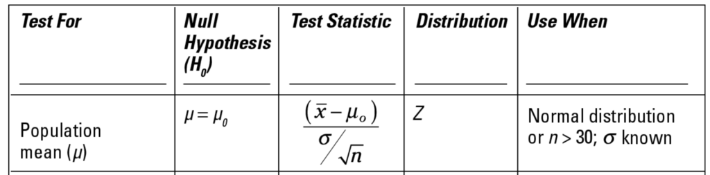
The last column, “Use when” states the assumptions that need to be in place for the test to work. We meet the normal distribution condition for both of these. However, we don’t have a known population standard deviation – we can only use the calculated standard deviation from our sample. So, we need to choose the t-test instead of the z test.
Step 6: Calculate the Z Score
This test uses the T distribution, and the Cheat Sheet tells us that and also gives us the formula for the t-statistic (test statistic). From here, we just plug in the numbers:
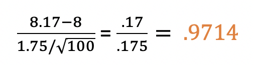
Our t-statistic is .9714.
Step 7: State Results
Check out this graph of the normal distribution, where the x axis is standard deviations. So, the 1 on the x axis means 1 standard deviation from the mean. The 0 means 0 standard deviations from the mean (which is the mean itself!)
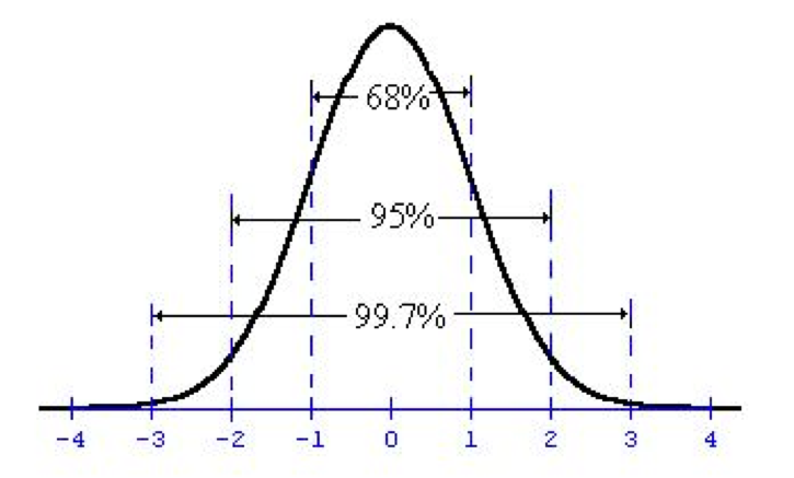
When you look at a chart like this for a hypothesis test, we’re always looking at it with the mean as the null hypothesis. So in this case, that 0 represents the 8. The 1 is one standard deviation away from the 8 ounces. Our Z score of .9714 falls about at the 1, which means the value 8.17 is about 1 standard deviation away from the mean. At 95% confidence, we can see from the chart that we need something 2 or more standard deviations away from the mean to reject the null hypothesis. Since we didn’t reach 2, we fail to reject the null hypothesis meaning that there is not sufficient evidence at the 95% confidence level that the average weight of the population is greater than 8 ounces. In other words, we don’t have enough evidence to conclude that the machines are overfilling the pies.
Optional Step 8: Calculate a P Value
You’ll hear p value thrown around a lot in statistics! The formal definition is the probability of getting an answer as extreme as the observed result if the null hypothesis is true. In other words, what’s the probability of getting 8.17 if the true average weight of the entire population of pies is 8 ounces? It’s also represented as the area between the curve and the x axis on that normal distribution graph above. As you can see, the further away from the mean (0) we get, the smaller the area between the curve and the axis, and thus the lower the probability of getting a result way out there.
We need a p-value calculator for to get the exact value. We recommend this one because it checks to see if you are doing a one or two-tailed test, and your confidence level. In our case, we’d type in .971 for the t-statistic and 99 for the DF value. DF stands for degrees of freedom, which is equal to the sample size (100 pies in our case) minus one. The significance level is 0.5 because we specified 95% confidence earlier in the test. And it’s a one-tailed test because our alternative hypothesis is greater than 8. If we chose “not equal to” 8 then it would be two-tailed.
The p-value is .166858 or 16.69%. This isn’t giving us any new information, it’s just another way of considering the t-statistic we got earlier. We need a p-value of less than 5% to reject the null hypothesis, and this is way higher than 5%, so we once again conclude that we fail to reject the null hypothesis at 95% confidence.
Optional Step 9: Confidence Intervals
As mentioned in my note earlier, these tests aren’t supposed to be exact, they’re giving a probability of getting a result assuming the null is true. Another way of thinking about this is that they are providing a range of values which, at 95% confidence, the true mean could lie within. If 8 is in that range, we fail to reject the null. If 8 is outside the range, we reject the null.
For our test, the range would be:
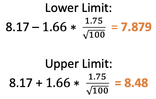
The number 8 is in this range, so we fail to reject the null at 95% confidence.
<< Previous Post
"Common Python Errors"
Next Post >>
"A/B Testing Example (Two Proportion Hypothesis Test)"